Next: 3 Interpolating Adaptive Data Up: Visualizing Data from Time-Dependent Previous: 1 Introduction

2 Adding Time-Dependency to Objects

  In this section we will briefly introduce our concept of time-objects.

 
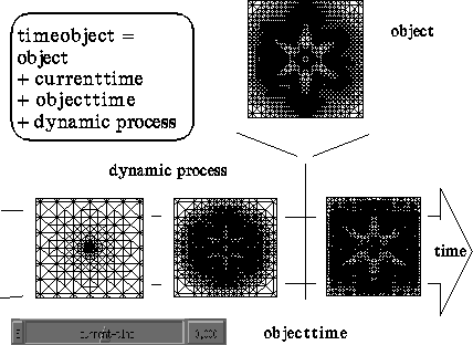
Figure 1:   A sketch of a time-object and the underlying dynamic process representing the simulation data. Here the growing of a dendrite is calculated on an adaptive triangular grid (A. Schmidt). The grid structure depicts the moving transition zone between the two phases.

More details can be found in [30]. Let us first refer to a simple but fundamental observation. Besides an appropriate projection and shading, it is mainly the interactive rotation, which makes an object appear three-dimensional on a flat screen. This can be transferred to time-dependent objects. The more flexibly we can manipulate and animate time and study arbitrary time cuts of dynamic processes, all the better we will understand the process as a whole. So it seems natural to build this flexibility directly into the corresponding structures, which we will call time-objects. In the frame discussed here, objects which depend on time may be points, curves and surfaces (for an application in the context of simulation data see section 4), or functions of finite element or finite volume type on an unstructured adaptive grid, for instance a tetrahedral mesh. Any of these objects can be extended to a time-object: We add a reference to a dynamic (process), an object-time and a current-time and define thereby a subclass of the object's class (cf. Fig.1).

 
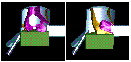
Figure 2:   Isosurfaces of the pressure of compressible gas flowing in a two stroke engine with a moving piston at two arbitrary times. The calculation is based on an adaptive and moving tetrahedral finite volume mesh (M. Wierse).

The object (or ancestral part) in such a time-object no longer represents a stationary data set, but a time cut of the underlying process dynamic at a time which is given by object-time. The variable current-time will in general be linked to some interactive control mechanism, for instance to a slider in a control panel. A typical structure for the process data dynamic (which is up to now a black box) will be inspected in the next paragraph. By the inheritance mechanism of OOP any previously implemented display method on the original object will immediately be available on the corresponding time-object. We achieve the necessary synchronization of the object-time with the current-time by the following simple update mechanism, which is invoked every time a message is sent to a time-object. It guarantees that always the current time cut of the dynamic process will be displayed.

if (current-time != object-time) {

where (dynamic "get-object") stands for the sending of the message "get-object" to the process dynamic.

At the level of the time-object there is only one thing essential for a correct working of this concept: The method get-object has to be implemented on the particular type of dynamic.

In GRAPE [42], our concrete environment, objects can be organized in a hierarchical structure so as to build a scene. The subscenes of this structure may represent time-dependent data. Therefore the underlying class scene has been enlarged to a time-scene as described above. The different current-time variables can now be controlled separately or can be synchronized. For that purpose, time-scenes additionally hold information on whether to synchronize with a global time or not. The actual synchronization is done by sending a synchronization message to the hierarchy. Then its time-scenes may align their respective current-times with the global time.

We've got two display strategies on a time-object. Applying some inherited method working on stationary data, we can flexibly display time cuts of the process (cf. Fig. 2). In addition, display messages can directly be sent to the dynamic process itself. For some important examples we refer to section 4.

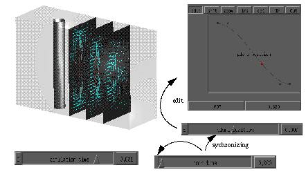
In interactive visualization, control panel components such as sliders, steer display parameters, positioning and rotation. Time-dependent geometric objects demand parameters which are time-dependent as well, i.e. a function over time. For example, cutting planes in a three-dimensional geometry with moving local phenomena such as vortex cores should move in accordance to the moving effects. We suggest to use time-sliders: By editing a spline representation of the attached function, we can modify the slider value over time. Visualization methods request for the current parameter value by sending a "get-object'' message to the time-slider, just as in the case of geometric objects (cf. Fig.3). The synchronization of control panels and geometry finally results in an arbitrary animation which can be adjusted interactively.

 
Figure:   A time-slider for the simulation time and a time-slider for the position of the cutting planes are synchronized with a main-time. The dependency on the main-time is described by an editable spline. Here the non-stationary viscous flow behind a cylindric obstacle (E. Bänsch) is visualized by plotting the velocity field on cutting planes. The colour represents the normal component.

Next: 3 Interpolating Adaptive Data Up: Visualizing Data from Time-Dependent Previous: 1 Introduction