Next: 4 A Framework for Up: Visualizing Data from Time-Dependent Previous: 2 Adding Time-Dependency to

3 Interpolating Adaptive Data

  Let's now turn to the question of how to handle dynamic processes consisting of adaptive simulation data.

Numerical simulation is in general a calculation of a list of successive time steps. On each time step the solution is given as a function on a mesh, which is evaluated best by a call , where singles out an element, and is a vector of local coordinates. For triangular or tetrahedral meshes we use barycentric coordinates as local coordinates, because most of the finite element functions, notably those of Lagrangian and Hermitian type, can easily be expressed in these coordinates [22][8].

The above mentioned "get-object" message requests for an interpolated solution at a certain time in between two time steps and . With the mesh fixed, it is obvious how to interpolate the two functions and that represent the numerical solution in and :

In the case of an adaptive strategy, the domain discretization will change from time step to time step. Therefore the function argument no longer corresponds to the same point on the two meshes, and their seems to be no straightforward interpolation mechanism. To bridge this gap, let us first briefly review the basics of an adaptive numerical strategy [21]. In a more abstract setting the partial differential equations governing the physical process under consideration turn out to be an ordinary differential equation in function spaces [29]

In addition has to fulfill appropriate initial and boundary conditions. Here is a nonlinear operator depending on the specific problem; e.g. applying the projection onto divergence-free functions to the Navier-Stokes system

,

for fluid velocity and pressure with the fixed force term , one just has to let

,

.

Adaptive solving now means to apply the following modification of some numerical ODE scheme. Given the post-adaption numerical solution on a grid at time , we calculate

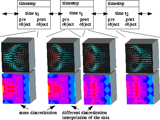
Here TimeStepEstimate returns the new step length; OneStep is a numerical scheme for the calculation of one time step, e.g. a backward Euler step [36]; AdaptMesh does the refining, coarsening or deforming of the current mesh according to heuristic criteria or a-posteriori error estimates; finally, the solution is transposed onto a new mesh by a Projection operator. At each time step this results in two pairs of solution and grid. Let us store the one as pre-object and the other as post-object in a structure time-step representing a time step at a certain time. Then we build a doubly linked list of these structures and end up with the appropriate data structure to settle a general interpolation mechanism (cf. Fig.4). We realize that the post-object of a time step and the pre-object of the successive time step are based on the same mesh, while pre-object and post-object of a single time step differ in the underlying grid, although the function is the same up to the projection. Therefore, on a list of time-steps, the message "get-object" causes a search for the right time interval; then the standard interpolation formula is applied in between post-object and pre-object of the two time-steps bounding the specific interval. Now we are able to inspect time dependent adaptive data interactively. In our experience, not the whole sequence of calculated solutions is necessary to achieve a continuous impression of the ongoing physical process. An a lot sparser list of steps will suffice.

 
Figure: Three time steps of a viscous flow in a rectangular container on an adaptive tetrahedral mesh (E. Bänsch) are depicted. Plane cuts with a mesh of vectors and a colour coding of the degree of refinement are drawn. The mesh width decreases from light blue to yellow.  

Let us finally remark that up to medium sized applications it might be possible to store the list of time steps in memory. For large data sets, one may replace the two objects of each time step by references to files on some disk. Then the "get-object" call will first have to load the requested objects and afterwards start the interpolation procedure. This approach can be improved combining both, direct storing and referencing, by a swapping mechanism for the time intervals currently of interest.

Next: 4 A Framework for Up: Visualizing Data from Time-Dependent Previous: 2 Adding Time-Dependency to