Next: 7 Conclusions Up: Visualizing Data from Time-Dependent Previous: 5 Algorithmic Aspects of
![]()
![]()
![]()
Next: 7 Conclusions Up:
Visualizing Data from Time-Dependent Previous:
5 Algorithmic Aspects of
Local properties of, say, a flow field ![]() and the related tensor
field
and the related tensor
field ![]() may be rendered by geometric symbols, which are placed at points of
interest (critical points, vortex cores etc.) [25][16][13]. Icons
assemble the local mathematical data and display-directives; a set of icons is
gathered in a linked list.
may be rendered by geometric symbols, which are placed at points of
interest (critical points, vortex cores etc.) [25][16][13]. Icons
assemble the local mathematical data and display-directives; a set of icons is
gathered in a linked list.
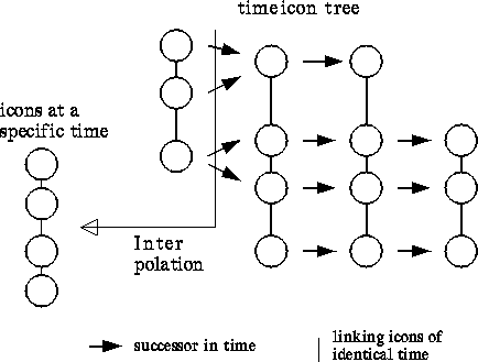
Figure 6: A sketch of the data
structure holding information on time-dependent icons. Each node corresponds to
a particular position in space and time; columns of nodes form time cuts;
horizontally linked nodes correspond to points of the (possibly forked) line in
space-time described by an icon.
Naturally, a time-dependent field requires mobile icons (cf. Fig. 7) that e.g. drift along particle paths or stay in the center
of a moving vortex, that arise, end, split and merge just as the inspected local
phenomena do. Such dynamic processes may be represented by time-icons: a
tree describes the evolution of a flock of ![]() . At each time-step we
have a list of icon nodes; each genuine node represents a particular icon at a
particular time (cf. Fig.6); it contains
. At each time-step we
have a list of icon nodes; each genuine node represents a particular icon at a
particular time (cf. Fig.6); it contains
Along each of those links that connect the successive states of an icon an
interpolation can be defined. Therefore, we can extract an interpolated list of ![]() at any
time in the time interval covered by the tree. And now, if the tree receives the
``get-object'' message, a linked list of icons is generated by
interpolation which then may be displayed.
at any
time in the time interval covered by the tree. And now, if the tree receives the
``get-object'' message, a linked list of icons is generated by
interpolation which then may be displayed.
While the movement of icons can be designed interactively, the generation of such a tree may be automated as well. A routine may string the subsequent steps of an icon on a given integral curve, or else one may apply a routine that identifies critical points.


Figure 7: Critical points in the
fluid flow behind a circular obstacle. The invariant subspaces of the saddle
(indicated by the arrows) converge as the vortex and the saddle come close. The
arrows point in the direction of the local flow.
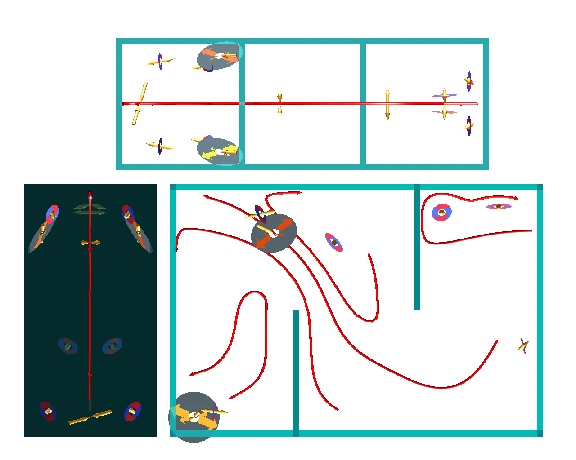
Figure 8: Critical points and
particle traces in a fluid container with inner walls. The arrows which are
scaled according to the eigenvalues of the gradient indicate the invariant
manifolds of the critical point; in the plane of the (grey) disk the point is a
node. The coloured disks describe the spiralling flow in the plane spanned by
the complex eigenvectors of the gradient.
![]()
![]()
![]()
Next: 7 Conclusions Up:
Visualizing Data from Time-Dependent Previous:
5 Algorithmic Aspects of