by Carsten Lange and Konrad Polthier
These animations show some experiments performed with our anisotropic fairing algorithm.
The images of each animation are consecutive snapshots. There was no post-processing neither of the images nor of the animations.
The connectivity of point sets is always computed from the point set alone, even if some of the initial point sets were produced from triangle meshes. Unless otherwise stated the connectivity is computed from the noisy initial point set and then fixed during the smoothing iteration.
Each video comes in two resolutions
- 640*512 (med)
- 320*256 (sml)
which differ by a factor of 4 in download time. SML videos vary in size between 100K and 1.4MB. The GIF animations should run at least with 10 frames per second, some sequences run at 20 frames per second. MED videos may run slower if either the video has not been fully downloaded yet or if the browser fails to refresh fast enough.
Denoising a Venus Torso ...
 |
 |
 |
 |
 |
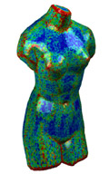
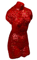
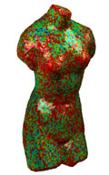
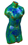
| Initial point set (68K) colored by maximal principal curvature. | 3% random normal and tangential noise | After 20 iterations | After 50 iterations | Varying point density in z-direction, different color range than left 4 images. |
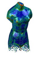
The Venus torso was subdivided to a resolution of 68K vertices and then disturbed with tangential noise to remove the visible subdivision patterns. All point sets are colored by their maximal principal curvature which is calculated from the point set.
The initial point set (a) was then further disturbed with a 3% normal and tangential noise to produce the initial noisy point set (b). Figures (c) and (d) show the point set after 20 respectively 50 steps of the anisotropic fairing algorithm. Figure (e) shows a denoised torso with varying point density in z-direction.
The lighting calculations use vertex normals parallel to the eigenvectors with smallest eigenvalue of the covariance matrix.
Zero Mean Curvature and Connectivity ...
 |
 |
 |
 |
| Tangential and normal noise added to a Costa minimal surface (5K). | After 20 iterations | After 50 iterations | After 50 iterations but during fairing the connectivity of the original point set was used. |
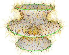
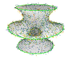
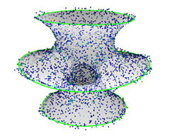
The smooth Costa surface is a minimal surface with both principles curvatures have equal absolute value and different sign. The points of a discrete Costa surface were randomly moved in normal and tangential direction with 3% noise (a). The vectors show the anisotropic mean curvature vector H whose length is also used for color coding of the vertices.
The connectivity of the point set is taken from the noisy initial point set (a) and kept fixed during the iteration. Figure (d) shows the result of 50 iterations when using the connectivity of the un-noised point set (which is still different than the original connectivity of the triangle mesh).
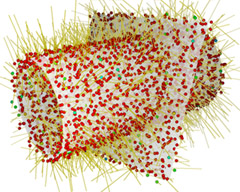
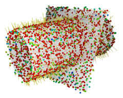
Intersecting Surfaces and Positive Mean Curvature
 |
 |
 |
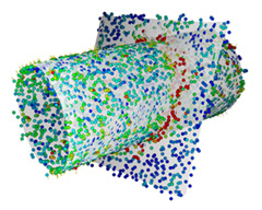 |
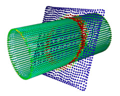
| Cylinder with constant positive mean curvature is intersected with plane. The point set consists of the union of both surfaces. | 3% tangential and normal noise added to the point set. Colored by length of anisotropic mean curvature vector. | After 15 iterations | After 50 iterations the planar area clearly shows zero mean curvature (blue) while the cylindrical area (greenish) still has non-vanishing H. |
Positive mean curvature leads to shrinking, and intersecting geometries have no well-defined principal curvature directions along the intersection line. Therefore this example demonstrates the behavior of our algorithm in two non-trivial test cases. Despite of the low resolution of the point set the positive mean curvature of the cylinder is recovered. The intersection line is recognized as an area of higher principal curvature and clearly separates the two areas, the curved cylinder and the flat plane.
Sharp Corners of a Solid
 |
 |
 |
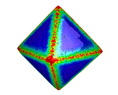 |
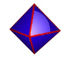
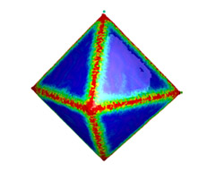
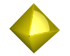
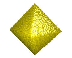
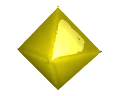
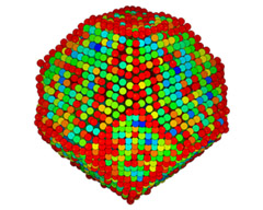
| Original octahedron with 32K vertices obtained from a 4-1 subdivision. | Initial point set with 1.5% tangential and normal noise. | Recovery of features and after 100 iterations with anisotropic MC flow. | Laplacian smoothing leads to lost sharpness of edges. |
The octahedron is a standard test case for anisotropic smoothing. Our algorithm recognizes and recovers sharp edges. Note the single vertex on top of the figure (c) which got stuck because all of its principal curvatures are above the curvature threshold.
Same Sequence with Lighting only ..
 |
 |
 |
| Original octahedron with lighting | Initial noise and lighting. | After 100 iterations the lighting looks pretty much recovered. |
The three figures show the same point sets as the previous row of figures but with lighting only. The coloring by principal curvature is replaced with a constant yellowish point color.
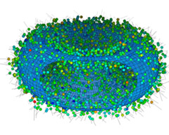
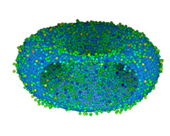
Influence of Connectivity
 |
 |
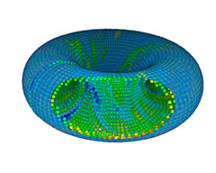 |
| Animation: (med,sml) |
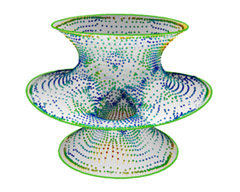
In contrast to most other sequences we compute the connectivity of the point set from the original uv-parametrized torus which is for convenience shown with reduced transparency as the underlying surface. Note, the connectivity is calculated from the original point set of the torus only, and it ignores the uv-mesh.
The right image shows how much of the original structure can be recovered if only the spatial adjacency of the original unnoised point set is known.
Low Resolution Model with Anisotropic MC Vector
 |
 |
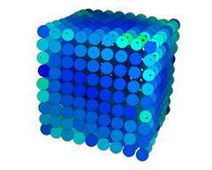 |
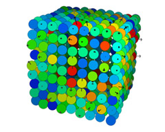
| Low resolution cube with 2.5% noise and anisotropic mean curvature vector. |
This example shows how the anisotropic mean curvature vector changes direction and length during an iteration on a low resolution model (<1K). The anisotropic shape operator recognizes the sharp edges and corner of the cube.
Truncated Octahedron with Different Sharp Edges
 |
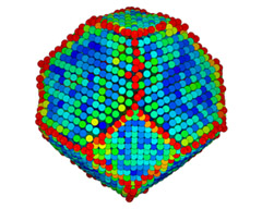 |
| Truncated octahedron with 2% noise colored by maximum principal curvature. | After 60 iterations the edges are clearly recovered as feature lines. |
The truncated octahedron has two type of edges with different dihedral angle. One set of edges has the same dihedral angle as an octahedron (109.47°) and the others (125.26°) are about 15° larger. This difference makes it harder to distinguish edges on a noisy version of the truncated octahedron.